Petroleum Engineering- Latest research

Pressure Drawdown Test Analysis: From Flow-Regime Identification to Reservoir Interpretation

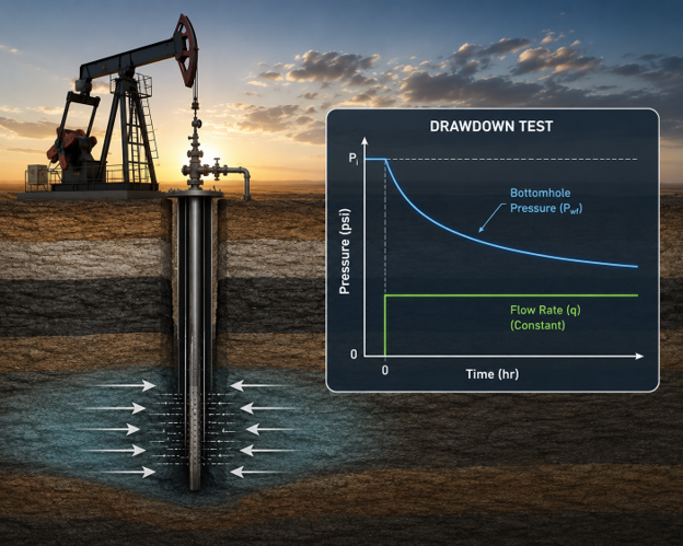
Pressure Drawdown Test Analysis showing a producing oil well, reservoir inflow toward the wellbore, declining bottomhole pressure, and constant production rate over time.

1. Introduction to Well Test Interpretation: The Inverse Problem

In the field of reservoir engineering, we are frequently tasked with solving an inverse problem. Unlike a forward problem where we know the reservoir model and predict the pressure response an inverse problem involves taking known system inputs (the flow rate history) and known outputs (the pressure response) to determine the unknown system: the reservoir itself.

As a technical educator, I must emphasize the critical distinction between analysis and interpretation. Analysis is the mechanical act of drawing lines on a graph to calculate numbers. Interpretation, however, is the high-level diagnostic process of identifying the physical nature of the reservoir. A pressure drawdown test is one of the fundamental pressure-transient testing methods used to characterize reservoir and near-wellbore behavior. It involves opening a well for production at an ideally constant rate after the reservoir has reached a uniform pressure.

An ideal drawdown test initiated from a stabilized reservoir and maintained at a constant production rate can be simpler to analyze than a test with a complex prior rate history. In field applications, however, rate fluctuations may require superposition or deconvolution techniques. This is due to the operational difficulty of maintaining a perfectly constant flow rate (q) during the initial production phase. However, when executed correctly, they provide the most direct look at the reservoir's undisturbed behavior.

2. Core Objectives of Drawdown Testing

The goals of transient drawdown testing are both quantitative and qualitative, focused on reducing the uncertainty inherent in the inverse problem.

  • Permeability (k): Determining the rock’s capacity to transmit fluid. This is often expressed as the permeability-thickness product (kh).
  • Skin Factor (s): Quantifying the degree of near-wellbore damage (from drilling/completion) or stimulation (from fracturing/acidizing).
  • Reservoir Boundaries and Connected Volume: Detecting boundaries and, when sufficiently late-time data and an appropriate reservoir model are available, estimating connected reservoir volume or drainage characteristics.
  • Deliverability: Establishing the well’s potential and long-term inflow performance.

Exploration vs. Development Testing

The "so what" of testing changes based on the well's lifecycle:

  • Exploration-Well Testing: The focus is on the entire reservoir. We ask: Is the prospect economically viable? How far do the boundaries extend? How much fluid is in place?
  • Development-Well Testing: The focus shifts to the individual well and the near-wellbore area. We use these tests to evaluate if a stimulation treatment was effective or if a well requires remedial work due to damage.

3. Assumptions and Limitations of Classical Drawdown Analysis

Classical pressure drawdown equations are derived from an idealized mathematical representation of fluid flow through porous media. Their direct application generally relies on several important assumptions:

  • Single-phase flow: Only one fluid phase is assumed to be mobile within the investigated reservoir region.
  • Slightly compressible fluid: Fluid density and volume change only slightly with pressure.
  • Darcy flow: The relationship between pressure gradient and flow velocity is assumed to remain linear.
  • Homogeneous reservoir: Reservoir properties such as permeability and porosity are assumed to be spatially uniform in the classical model.
  • Constant fluid and rock properties: Parameters such as https://glossary.slb.com/en/terms/p/pressure_transient_analysis?utm_source=chatgpt.comviscosity, compressibility, permeability, and formation volume factor are assumed to remain constant during the test.
  • Constant production rate: The ideal drawdown solution assumes that the well is produced at a constant rate from the beginning of the test.
  • Adequate test duration: The test must continue long enough for the pressure transient to investigate the reservoir region and develop the flow regimes required for interpretation.

Real reservoirs and field operations, however, rarely satisfy all of these assumptions perfectly. Deviations from ideal conditions can significantly alter both the pressure response and the pressure derivative.

Multiphase flow, for example, introduces saturation-dependent relative permeability and mobility changes, meaning that the observed pressure response may no longer represent a simple single-phase diffusivity process. Phase redistribution within the wellbore can generate complex early-time behavior and may be confused with conventional wellbore-storage effects.

Similarly, changing production rates distort the pressure response because the measured pressure at any time reflects the cumulative effect of the previous rate history. In such cases, simple constant-rate drawdown equations may become inadequate, and techniques such as superposition, rate normalization, or deconvolution may be required.

Other non-ideal behaviors can also produce characteristic or overlapping diagnostic responses. Non-Darcy flow, particularly in high-rate gas wells, introduces additional rate-dependent pressure losses. Hydraulic or natural fractures may generate linear or bilinear flow before radial flow develops. Dual-porosity reservoirs can exhibit transition behavior associated with fluid exchange between the matrix and fracture systems. Pressure-dependent rock and fluid properties may violate the constant-property assumptions underlying conventional analytical solutions.

Finally, gauge resolution, measurement noise, rate uncertainty, and insufficient test duration can obscure derivative features and lead to ambiguous model identification. Because the pressure derivative is particularly sensitive to data quality and numerical differentiation, apparent flow regimes should never be identified solely from a short or noisy derivative trend.

Therefore, classical drawdown equations should be viewed as model-based interpretation tools rather than universally exact descriptions of reservoir behavior. Reliable well-test interpretation requires the analyst to identify where the assumptions of the selected model are valid, recognize deviations from ideal behavior, and integrate pressure-transient data with rate history, completion information, PVT data, geological knowledge, and other available reservoir information.

4. Analysis Methodology I: Radial Flow Semilog Analysis

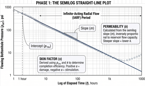
The "Straight-Line Method" remains a fundamental technique for identifying Infinite-Acting Radial Flow (IARF). During IARF, the pressure transient expands radially into the reservoir, and the pressure response follows a logarithmic relationship with time.

Plotting Pwf vs. log(time) identifies the IARF period for primary flow capacity analysis.

Visual Analysis Guide: The Semilog Plot

An analyst should plot pressure (P) on a linear y-axis against time (t) on a logarithmic x-axis.

  • The Logarithmic Axis: This scale is essential for expanding early-time data. Consultant’s Rule of Thumb: To quickly estimate distances on the fly, remember that one-half of a log cycle is approximately a factor of 3 (e.g., from 1 to 3), and one-third of a log cycle is approximately a factor of 2 (e.g., from 1 to 2).
  • Identifying the Straight Line: The straight line only exists during the IARF period. Any data prior to this is likely distorted by Wellbore Storage (WBS) and must be ignored for slope calculations.
  • Slope (m): The slope of the straight line is inversely proportional to kh. A steeper slope indicates lower permeability for a given thickness and rate.
  • P1hr: We use the pressure value on the extrapolated straight line at 1-hour P1hr to calculate the Skin Factor. This value represents the deviation from an ideal, undamaged state.

Wellbore Pressure Equation: Pwf (t)=pi−162.6qBμ/kh [log(t)+log(k/(ϕμc_t r_w^2 )−3.23+0.869s]

Semilog Straight-Line Slope (m): m=− 162.6qBμ/kh

Permeability: k=162.6qBμ/(∣m∣h)  

Skin Factor: s=1.151[((pi-p1hr)/(∣m∣))− log (k/(ϕμc_t r_w^2 ))+3.23]

Radius of Investigation (ri): ri=√(kt/(948ϕμc_t ))

  • q: STB/day
  • B: rb/STB
  • μ: cp
  • k: md
  • h: ft
  • t: hr
  • rw: ft
  • ct: psi−1
  • Pressure: psi

5. Analysis Methodology II: Log-Log Diagnostic Plotting

Modern interpretation relies on the "Diagnostic Plot," which uses the Gringarten-Bourdet pressure derivative (P') to identify the reservoir model with far greater precision than semilog plots alone.

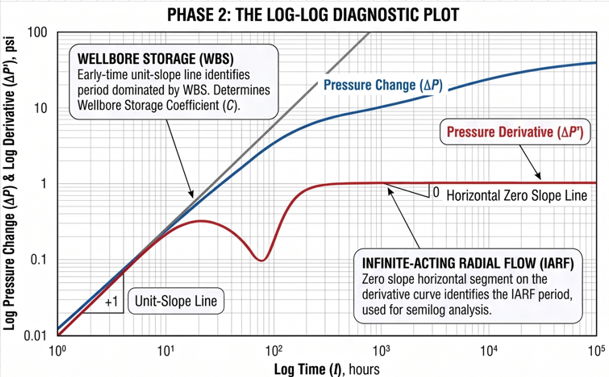
Graphs pressure change and derivative vs. time on log-log scales to identify distinct flow regimes.

Visual Analysis Guide: The Diagnostic Plot

This plot features both the pressure change (∆P) and the derivative (∆P') on a log-log scale.

  • Wellbore Storage (WBS) Region: Identified by a unit-slope straight line (45-degree angle) at early times on both the ∆P and ∆P' curves. This represents fluid expansion within the wellbore itself, not the reservoir.
  • Infinite-Acting Radial Flow Region: This is the most critical diagnostic feature. It is identified by a horizontal plateau (zero-slope) on the pressure derivative curve.
  • The kh Calculation: Crucially, it is the vertical position of this plateau on the y-axis that allows the analyst to calculate the kh product directly.
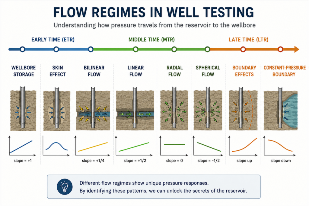
  • How Skin Appears in the Pressure Response: The skin factor represents an additional pressure drop—or, in some cases, a pressure gain—associated with flow conditions in the near-wellbore region. However, skin should not generally be interpreted as an independent flow regime. Unlike wellbore storage, radial flow, linear flow, or boundary-dominated behavior, skin primarily modifies the magnitude of the pressure response rather than producing a unique diagnostic derivative signature. A positive skin factor indicates additional flow resistance near the wellbore, whereas a negative skin factor generally indicates improved well productivity relative to the ideal radial-flow condition. However, positive skin should not automatically be interpreted as formation damage. The observed or apparent skin may result from several physical and completion-related effects, including drilling-induced damage, partial penetration, limited perforation efficiency, completion geometry, scale deposition, fluid blockage, and other near-wellbore restrictions. In gas wells, rate-dependent non-Darcy flow can also contribute significantly to the apparent skin.

The pressure response associated with skin must therefore be interpreted together with wellbore storage and the transition toward reservoir-dominated flow. At early time, wellbore storage may mask the reservoir response and prevent reliable estimation of skin. Skin calculations performed before a clear IARF regime has developed can therefore produce misleading results.

For this reason, the analyst should first identify the relevant flow regimes using the pressure derivative, confirm the radial-flow period, and only then estimate skin using an appropriate analytical or model-based method. The calculated skin should subsequently be evaluated in the context of the well’s completion design, stimulation history, production conditions, and geological setting. In practice, skin is not merely a numerical parameter; it is the combined pressure signature of processes occurring in and around the near-wellbore region.

Pressure Equation: = (p_i-p_wf (t))/(q(t))= 162.6Bμ/kh[logt+log⁡(k/(φμc_t r_w^2 ))-3.23+0.869s]

Permeability: k= 162.6Bμ/m'h  (where m′ is the slope of the rate-normalized pressure plot)

​ Skin Factor: s=1.151[((Δp/q)1hr)/m') − log ((k/(ϕμc_t r_w^2 ))+3.23]

 6. The Necessity of Integrated Interpretation

Because well testing is an inverse problem, the solutions are often non-unique. Several different reservoir models can produce the same pressure response on a single plot. To reduce this uncertainty, the analyst must use Integrated Interpretation, viewing data across Cartesian, semilog, and log-log scales simultaneously.

  • Cartesian plots are excellent for identifying late-time boundary effects or pressure depletion.
  • Semilog plots confirm the IARF period used for k and s calculations.
  • Log-Log plots are the primary diagnostic tool for model identification.

Relying on one scale leads to "hidden behavior" for example, a Cartesian plot often hides early-time damage because the data is compressed against the y-axis. Only by ensuring the model honors all scales can we move to the final step: Simulation and History Matching. In this stage, we use the kh and s estimates from our analytical methods as the starting point for a numerical simulator. We then fine-tune the model until the simulated response matches the field data, ensuring our interpretation is physically grounded.

 7. Conclusion and Summary: The Reservoir Engineer’s Workflow

Parameter estimates are meaningless if the underlying reservoir model is incorrectly identified. Follow this disciplined workflow:

  1. Collect and QC Data: Verify flow rates and pressure gauge accuracy.
  2. Identify Flow Regimes: Use the diagnostic plot to find WBS, IARF, and boundaries.
  3. Select the Reservoir Model: Ensure the selected model is consistent with the geology and logs.
  4. Estimate Parameters: Calculate kh, s, and reservoir volume using appropriate methods.
  5. Validate Results: Use history matching to confirm the model's accuracy across all time scales.

Key Takeaways:

  1. Model identification must precede parameter estimation.
  2. Errors in ct and h are the most common sources of major volumetric miscalculations.
  3. Always check for WBS distortion on the semilog plot before trusting the slope m.


Leave a Reply

Your email address will not be published. Required fields are marked *