Understanding Flow Regimes in Pressure Transient Analysis: A Practical Guide to Well Test Interpretation
1. Introduction: Why Flow-Regime Identification Comes First
Pressure transient analysis (PTA) is fundamentally an inverse problem. The reservoir itself cannot be directly observed during a well test; instead, engineers record changes in pressure and flow rate and use these responses to infer the underlying reservoir structure, flow geometry, boundaries, and near-wellbore conditions.
This is why flow-regime identification must precede parameter estimation. A permeability value calculated from the wrong flow regime may be mathematically correct but physically meaningless.
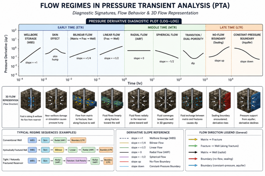
Modern well test interpretation therefore relies heavily on the log-log diagnostic plot, where pressure change (Δp) and pressure derivative (Δp′) are plotted against elapsed time. Different flow geometries generate characteristic derivative responses, allowing the analyst to recognize how pressure disturbance propagates through the well-reservoir system.
However, these signatures should not be treated as rigid templates. Real pressure responses may be distorted by wellbore storage, skin, changing rates, multiphase flow, reservoir heterogeneity, gauge noise, and overlapping flow regimes. Interpretation therefore requires both pattern recognition and physical reasoning.

2. Reading the Diagnostic Plot
The pressure derivative is commonly expressed conceptually as:
∆p'=(d(∆p))/(d lnt )
The derivative emphasizes changes in the pressure response that may be difficult to recognize on conventional Cartesian or semilog plots.
A useful principle is:
The shape and slope of the pressure derivative reflect the geometry and physics of fluid flow in the reservoir.
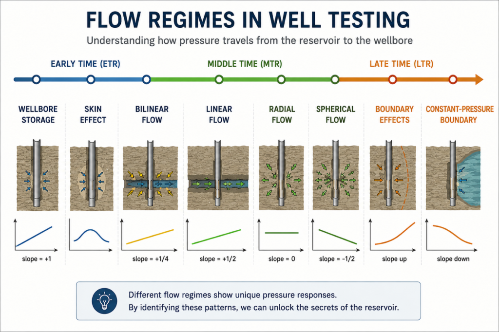
A horizontal derivative may indicate radial flow, while positive or negative derivative slopes can indicate linear, bilinear, spherical, storage-dominated, or boundary-influenced behavior.
For practical interpretation, the test response can often be divided into three broad time regions:
- Early time: dominated by the wellbore, completion, fractures, and near-wellbore effects.
- Intermediate time: often contains reservoir flow regimes used to estimate properties such as permeability and skin.
- Late time: may reveal reservoir boundaries, connected volume, interference, or external pressure support.
These time regions are conceptual rather than fixed. A particular flow regime may appear earlier or later depending on reservoir properties, well geometry, completion, and test duration.
At the beginning of a pressure transient test, the measured response may primarily reflect fluid expansion, compression, or movement within the wellbore rather than flow from the reservoir.
For ideal wellbore storage
∆p ∝ t
Therefore, both the pressure changes and pressure derivative exhibit approximately a unit slope on the log-log diagnostic plot.
Diagnostic signature
Derivative slope≈+1
During this period, the downhole sandface rate may differ significantly from the measured surface rate. Consequently, reservoir parameters should generally not be estimated from data dominated by wellbore storage.
The transition away from wellbore storage can also contain information about skin and near-wellbore effects, but the shape of this transition should not automatically be interpreted as a separate reservoir flow regime.
4. Infinite-Acting Radial Flow (IARF)
Infinite-Acting Radial Flow is one of the most important flow regimes in conventional well test analysis.
During radial flow, fluid converges toward the well approximately radially in the horizontal plane. The pressure response becomes logarithmic with time, producing a straight line on a semilog pressure-versus-time plot.
On the log-log diagnostic plot, the defining feature is a horizontal pressure-derivative plateau:
(d(∆p))/(d logt ) ≈0
Horizontal derivative plateau — zero slope
The term infinite-acting does not mean that the reservoir is physically infinite. It means that, during the observed time interval, the pressure transient has not yet encountered a boundary that significantly affects the measured response.
The radial-flow regime is particularly important because it is commonly used to estimate:
A short flat section should not automatically be classified as radial flow. The analyst should verify that the response is consistent across the log-log, semilog, and other relevant plots.
5. Linear Flow
Linear flow occurs when fluid moves predominantly along approximately parallel flow paths toward the well or fracture.
It is commonly associated with:
- Hydraulically fractured wells
- Long horizontal wells under certain conditions
- Channelized reservoirs
- Geometrically constrained flow systems
For ideal linear flow:
∆p ∝ t^(1⁄2)
Therefore, the pressure derivative exhibits a characteristic:
Derivative slope=+ 1/2
Diagnostic signature
Half-slope (+1/2) derivative trend
The presence of linear flow can provide important information about fracture behavior and effective flow geometry. However, a 1/2-slope trend should be interpreted together with the completion geometry and geological model because different physical systems can generate similar transient signatures
Bilinear flow is particularly important in the analysis of finite-conductivity hydraulic fractures.
During this regime, two flow processes occur simultaneously:
- Reservoir fluid flows toward the fracture.
- Fluid flows along the fracture toward the wellbore.
This coupled flow behavior produces the characteristic relationship:
∆p ∝ t^(1⁄4)
and therefore:
Derivative slope=+ 1/4
Diagnostic signature
Quarter-slope (+1/4) derivative trend
Bilinear flow may indicate that the fracture has finite conductivity and that pressure losses along the fracture itself are significant.
The distinction between 1/4-slope bilinear flow and 1/2-slope linear flow is therefore important for evaluating the behavior of stimulated wells.
7. Spherical and Hemispherical Flow
Spherical flow develops when fluid converges toward the producing interval in three dimensions rather than flowing predominantly in a horizontal radial plane.
This behavior may occur in situations involving:
- Partial penetration
- Limited completion intervals
- Restricted vertical communication near the well
- Certain completion geometries
For ideal spherical flow, the pressure derivative commonly exhibits a characteristic negative trend approaching:
Derivative slope=- 1/2
Hemispherical flow may occur when the geometry restricts the flow domain to approximately half of a spherical system.
8. Fracture-Related Flow Regimes
Hydraulically fractured wells may exhibit several successive flow regimes rather than a single fracture signature.
Depending on fracture conductivity, geometry, reservoir permeability, and test duration, the response may progress through:
Wellbore Storage → Bilinear Flow → Linear Flow → Radial Flow
Not every test will display all of these regimes clearly.
For example:
- A finite-conductivity fracture may produce bilinear flow.
- A sufficiently conductive fracture may exhibit a clearer linear-flow regime.
- At later time, the pressure disturbance may eventually extend beyond the fracture-dominated region and develop radial flow around the effective well-fracture system.
Therefore, fracture interpretation should be based on the sequence and duration of flow regimes, not on a single derivative slope alone.
Naturally fractured reservoirs may contain two interacting pore systems:
- A relatively high-conductivity fracture network
- A higher-storage but lower-conductivity rock matrix
Under appropriate conditions, the pressure derivative can display a characteristic transition or dip between two flow periods.
This behavior reflects fluid exchange between the matrix and fracture systems.
However, an important interpretation warning is required:
A derivative dip is not automatically proof of a dual-porosity reservoir.
Similar features may be produced by other mechanisms, including:
- Layered reservoirs
- Composite systems
- Changing mobility
- Multiphase effects
- Rate-history distortion
The pressure response must therefore be evaluated together with geological, image-log, core, and completion information.
10. Channel and Geometrically Confined Flow
A reservoir bounded by approximately parallel no-flow boundaries may eventually behave as a channel.
After the pressure transient interacts with both boundaries, the effective flow geometry can become predominantly linear.
The derivative may therefore develop a positive trend resembling a half-slope response.
This creates an important interpretation challenge: both a hydraulic fracture and a channelized reservoir can produce linear-flow signatures.
The distinction must be made using:
- The time at which the regime appears
- The preceding flow regimes
- Well and fracture geometry
- Geological information
- Boundary orientation
- History matching
This demonstrates why derivative slope alone cannot uniquely determine the reservoir model.
11. No-Flow Boundary Response
A sealing fault or closed reservoir boundary prevents fluid flow across the boundary.
When the pressure transient reaches a single sealing boundary, the pressure derivative begins to rise above the original radial-flow plateau. Under ideal conditions, a single no-flow boundary may eventually produce a derivative stabilization at approximately twice the original radial-flow level, consistent with the image-well concept.
More complex closed geometries may generate stronger late-time responses.
Diagnostic behavior
Late-time derivative upturn
Potential causes include:
- Sealing faults
- Closed reservoir boundaries
- Intersecting boundaries
- Finite drainage regions
However, not every derivative upturn represents a physical boundary. Rate changes, multiphase behavior, and data-quality problems can also distort late-time data.
12. Constant-Pressure Boundary
A constant-pressure boundary maintains pressure support as the transient approaches it.
Possible physical examples include:
- Strong aquifer support
- Pressure-maintained boundaries
- Certain communication systems
The pressure derivative typically shows a late-time downturn, eventually tending toward lower values under ideal constant-pressure behavior.
Diagnostic behavior
Late-time derivative downturn
This behavior contrasts with the upward response commonly associated with a no-flow boundary.
If the reservoir is finite and effectively closed, the pressure transient may eventually investigate the entire connected drainage volume.
At this stage, the system no longer behaves as an infinite-acting reservoir, and late-time pressure behavior becomes controlled by the finite reservoir volume and boundary configuration.
This region may provide information about:
- Connected reservoir volume
- Drainage area
- Boundary configuration
- Reservoir compartmentalization
Reliable volumetric interpretation, however, requires sufficiently long test duration and appropriate estimates of porosity, total compressibility, net thickness, and fluid properties.
14. How Skin Appears in the Pressure Response
The skin factor represents additional pressure loss—or pressure improvement—associated with the near-wellbore region and completion system.
Skin is generally not an independent flow regime with a universal derivative slope.
A positive skin factor may result from:
- Formation damage
- Partial penetration
- Inefficient perforations
- Completion restrictions
- Scale or fluid blockage
- Near-wellbore alterations
- Rate-dependent non-Darcy effects
Therefore:
s>0≠formation damage only.
Similarly, negative skin may indicate stimulation or an effective completion geometry that improves well productivity.
Because early-time behavior may be dominated by wellbore storage, skin should be estimated only after the analyst has identified an appropriate reservoir flow regime and selected a physically consistent model.
15. Flow-Regime Sequences Are More Important Than Isolated Shapes
One of the most important principles in modern PTA is that the sequence of flow regimes often contains more diagnostic information than any individual slope.
For example:
WBS→Bilinear Flow→Linear Flow→Radial Flow→Boundary Response
may suggest a very different physical system from:
WBS→Bilinear Flow→Linear Flow→Radial Flow→Boundary Response
The analyst should therefore ask:
What physical reservoir model can explain the entire pressure response—not just one section of the derivative curve?
16. Why Flow-Regime Identification Can Be Ambiguous
Real well-test data rarely display perfect textbook signatures. Flow regimes can overlap, disappear, or become distorted because of:
- Wellbore storage
- Phase redistribution
- Variable production rates
- Multiphase flow
- Non-Darcy flow
- Reservoir heterogeneity
- Natural and hydraulic fractures
- Pressure-dependent properties
- Gauge noise
- Insufficient test duration
For example, a short apparent 1/2-slope derivative trend could potentially represent fracture linear flow, channelized flow, or simply a transition between two other regimes.
Therefore, pattern recognition alone is insufficient.
A reliable interpretation should combine multiple diagnostic views:
Log-log diagnostic plots are used primarily for flow-regime identification.
Semilog plots help confirm radial flow and support conventional permeability and skin calculations.
Cartesian plots can reveal overall pressure trends, depletion behavior, and certain late-time responses.
The final interpretation should also be consistent with:
- Well completion geometry
- Geological model
- PVT properties
- Production history
- Core and log information
- Known faults and reservoir boundaries
Once a physically plausible model has been selected, analytical estimates can be used as initial parameters for simulation and history matching.
Conclusion
Flow-regime identification is the foundation of pressure transient interpretation. Characteristic derivative behaviors—such as the unit slope of wellbore storage, the horizontal plateau of radial flow, the half slope of linear flow, and the quarter slope of bilinear flow—provide powerful clues about the physics of the well-reservoir system.
However, a derivative signature is evidence, not proof.
Different reservoir models may generate similar pressure responses, and real field data are often affected by overlapping physical processes. The objective of the reservoir engineer is therefore not simply to match a curve to a textbook pattern, but to identify a physically consistent reservoir model that explains the complete pressure response across all relevant time scales.
Key Takeaways
- Identify the flow regime before calculating reservoir parameters.
- Use derivative slopes as diagnostic evidence, not as standalone proof of a reservoir model.
- Interpret the sequence of flow regimes rather than isolated curve shapes.
- Distinguish early-time well and completion effects from true reservoir behavior.
- Validate the interpretation using multiple plots, geological information, and history matching.